Optimise a striatal fast-spiking interneuron¶

This Use Case demonstrates how BluePyOpt can be used to optimize a striatal fast-spiking interneuron. The notebook is self-contained and runs a few steps of the genetic optimization. For a production run, the population size as well as the number of iterations need to be increased as commented in the notebook.

The notebook starts by downloading the relevant code from the Collab storage and setting up the simulation and graphical environment. Since we are using Neuron, we also need to compile the channel mod files.

The information about the optimization to be run is stored in config/ directory:

• protocols.json

• features.json

• mechanisms.json

• parameters.json and parameters-demo.json

For each set of parameters to be tested a neuron model is instantiated by the evaluator. A series of current injections is sent to the neuron while recording the somatic voltage. A number of features are extracted from this voltage trace, and compared to the same features extracted from the corresponding experimental data.

protocols.json lists the protocols and the associated stimuli. Each protocol also specifies a holding current. The delay, amplitude, duration and total duration are specified for each current injection.

features.json lists the features. Each protocol has its own set of features. For each feature the mean value and standard deviation (SD) are specified. The SD is used when weighting the feature scores together to get the final score for the model. Each feature also has a set of modifying parameters.

mechanisms.json lists the mechanisms. Each ion channel has a corresponding mod file which is compiled by nrnivmodl.

parameters.json lists all the model parameters. These can either be specified as a value, or as a range, by giving its upper and lower bounds.

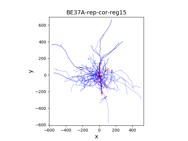
Morphology of the neuron is located in morphology/ directory:

• morphology/BE37A-rep-cor-reg15.swc

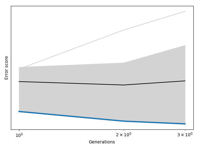
The optimization phase is followed by the post optimization analysis within the same notebook. The script plots the evolution of the error scores with successive iterations of the genetic algorithm (generations).

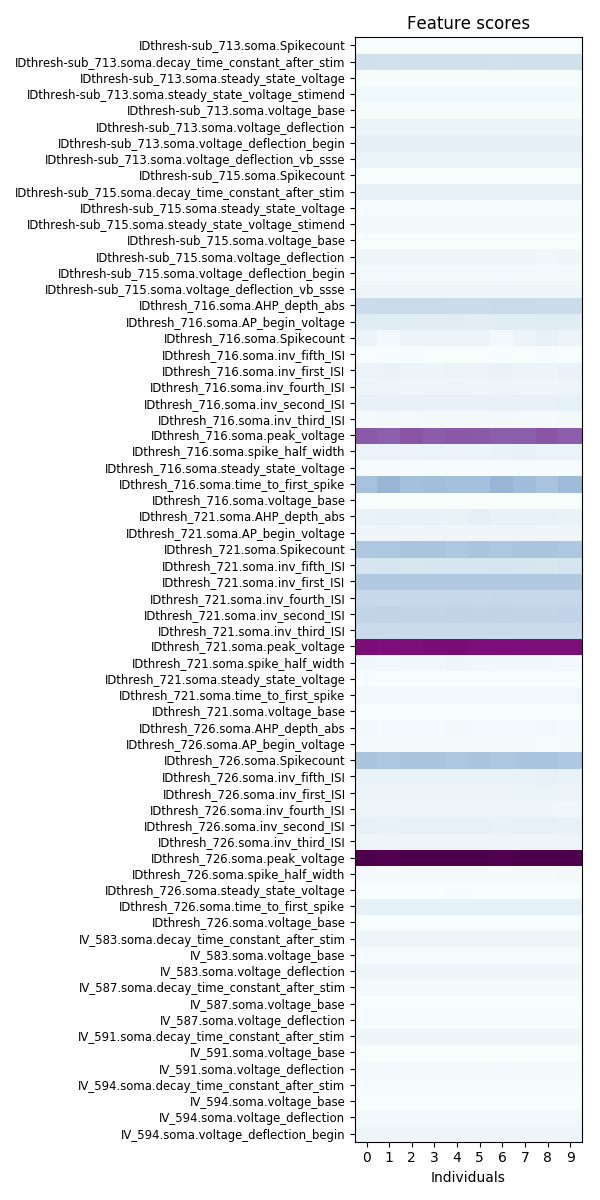
It displays the top ten individuals with the best scores and lists the feature names.

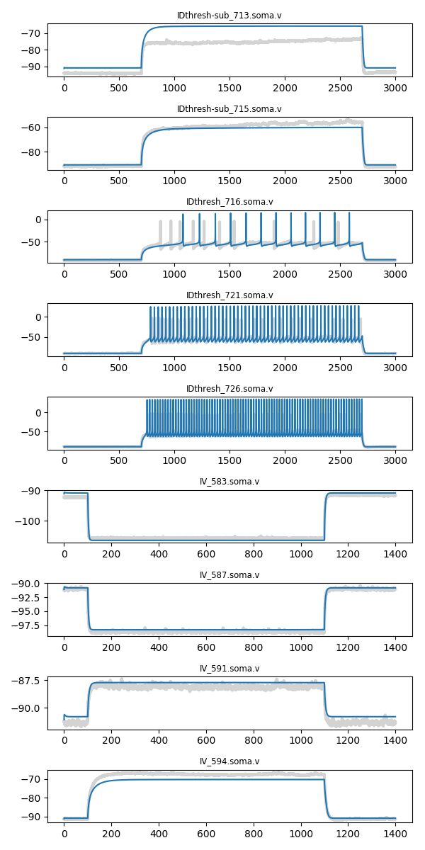
It also displays the simulated protocols (blue) overlaid on the experimental data (grey) for the best individual.

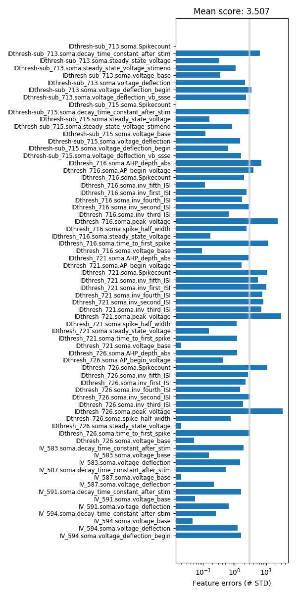
Finally, errors for each feature of the best individual are shown and also a mean error score is calculated. Typically, the mean score is about 3 standard deviations.

It is possible to inspect any of the 10 candidate individuals as shown above for the best individual. Corresponding instructions are given in the notebook.