Subcellular application
The subcellular application and molecular repository were developed as a software environment for simulation of brain molecular networks.
It was designed to reach several objectives related to major restrictions of currently available software tools, such as the lack of integration with existing biological data relevant for modeling and the low compatibility of different types of models.
General info
The subcellular application was designed as a hub web based environment for creation and simulation of reaction-diffusion models integrated with the molecular repository. It allows also to import, combine and simulate existing models expressed with BNGL and SBML languages.
Two types of models are supported: rule-based models convenient and computationally efficient for modeling big protein signaling complexes and chemical reaction network models.
The subcellular application is integrated with a number of solvers for reaction-diffusion systems of equations. It supports simulation of spatially distributed systems using STEPS (stochastic engine for pathway simulation) – which provides spatial stochastic and deterministic solvers for simulation of reactions and diffusion on tetrahedral meshes.
The application provides as well a number of facilities for visualizing the models geometry and the results of the simulations.
The molecular repository is a publicly available database of biological information, relevant for brain molecular network modeling.
It accommodates several types of biological information which are not available from existing public databases, such as concentrations of proteins in different subcellular compartments of neuronal and glial cells, kinetic data on protein interactions specific for brain and synaptic signaling and plasticity, data on molecules mobility.
The repository is integrated with the subcellular application. They share the same set of entities described by BioNetGen expressions. The molecular repository can be queried from the subcellular application and the results of the query can be added to a molecular network model.
Usage
Open subcellular application by using this link: SubcellularApp
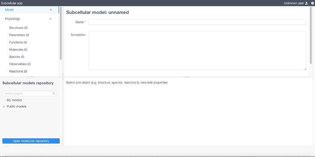
Create a new model or load/import an existing one
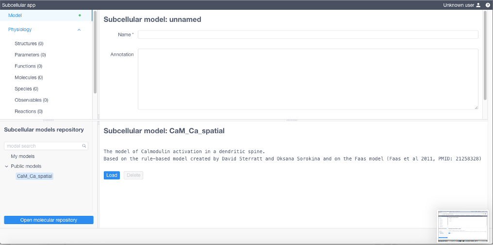
To load a public model click the arrow to expand a list of public models in Subcellular models repository, choose one, then click Load
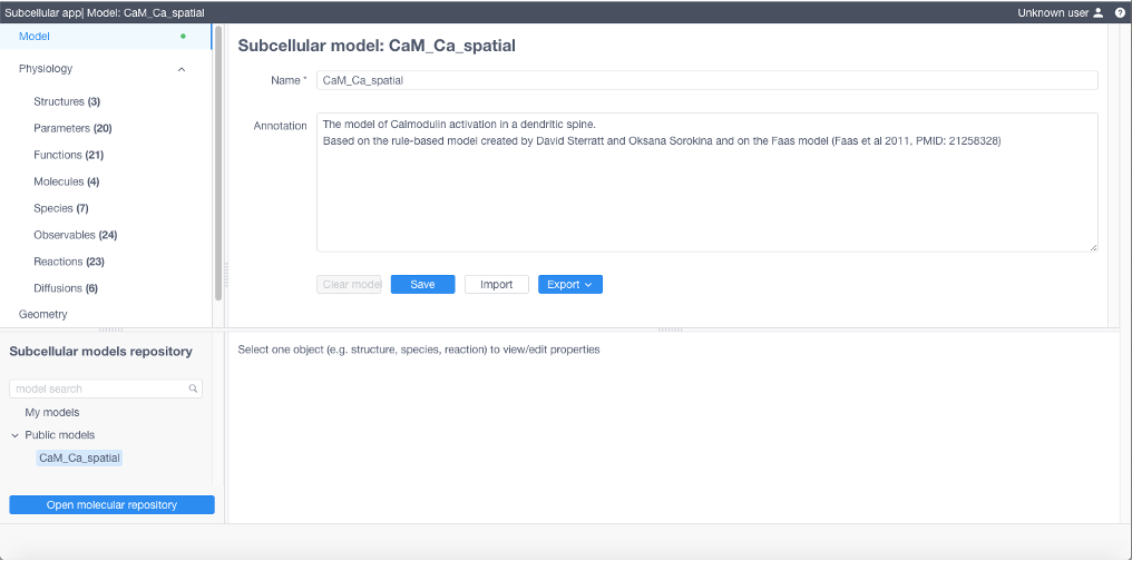
To create a new model specify all model parameters and reaction equations sequentially opening and filling the tables in the Model menu (upper left of the UI). Each table corresponds to a particular section of the BioNetGen file of the model (with except for Diffusions and Geometry section). All expressions should comply with the BioNetGen language.
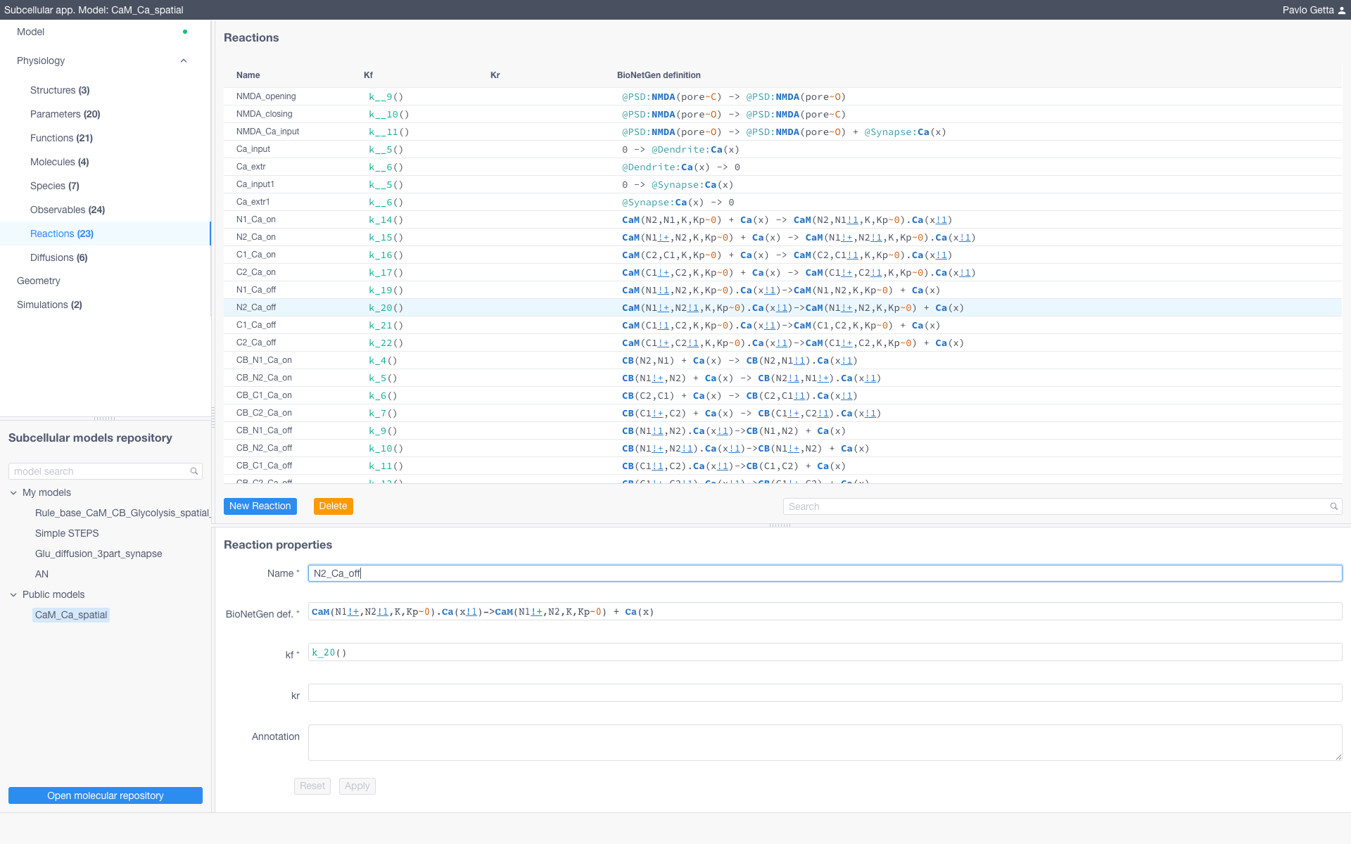
Models are represented by a set of structures (e.g. compartments of models) and a collection of entities from the BioNetGen language such as parameters, functions, molecules, species, observables and reactions. To modify these entities sof the model navigate to the corresponding section in the Physiology dropdown menu and specify them according to the BioNetGen language (for more about BioNetGen see the official documentation)
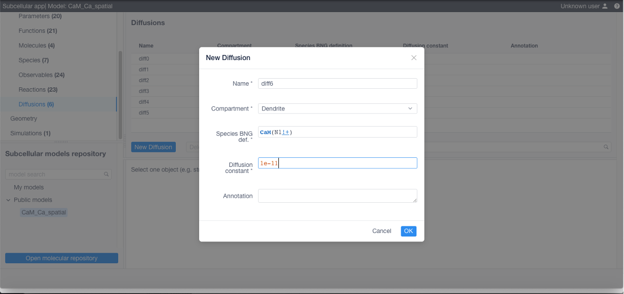
To add diffusions (required if using STEPS) navigate to the corresponding section, click New diffusion and specify a name for the diffusive species or molecules, the affected structure, the BNGL expression and the diffusion coefficient in m^2/s.
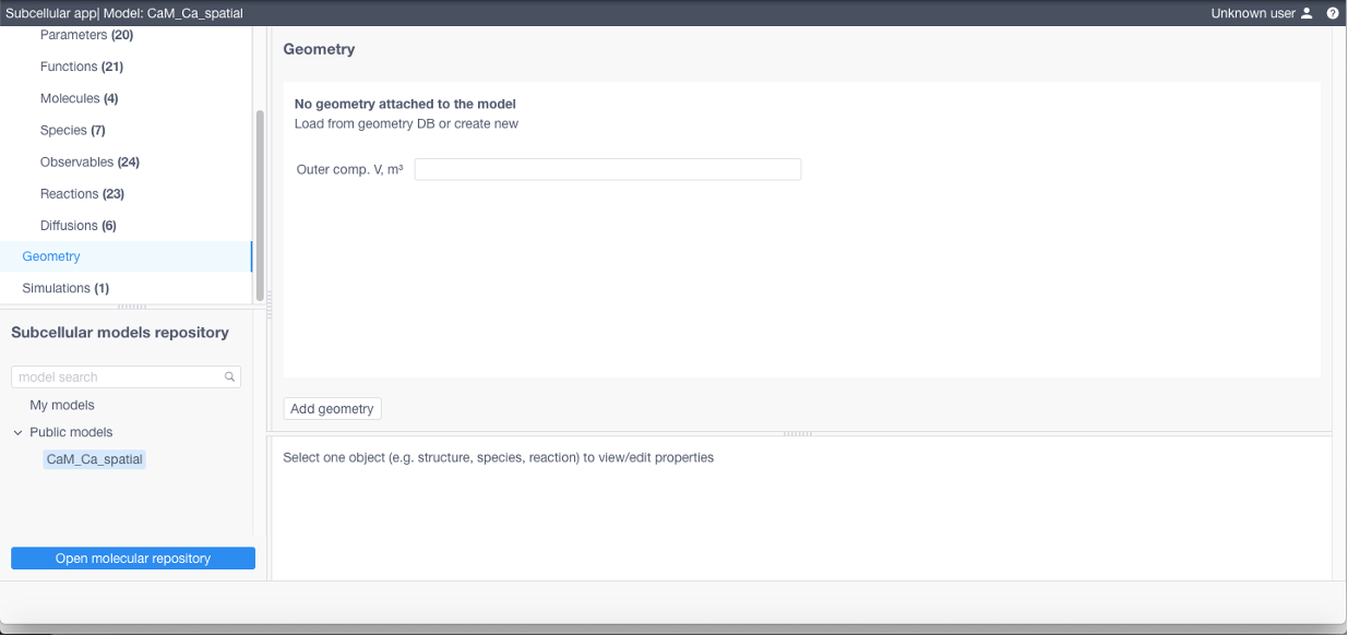
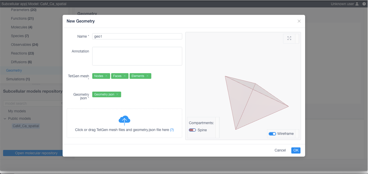
To add a geometry (required if using STEPS) click Add geometry in the corresponding section: specify its name, add a TetGen tetrahedral mesh and a geometry specification file (geometry.json, contains relationship between structures and their corresponding tetrahedra and triangles, free diffusion boundaries and geometry scale coefficient converting mesh vertices position units to meters, see examples below)
At any stage model can be:
saved using Model -> Save sequence, and then loaded from My models in Subcellular models repository
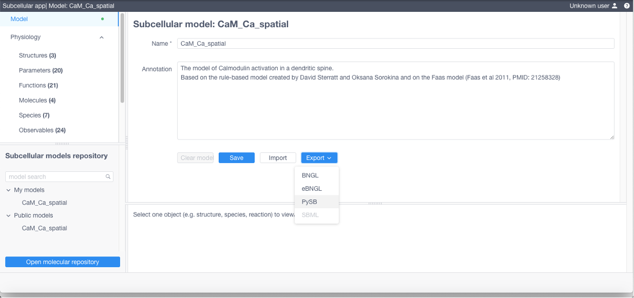
exported into different formats by using Model -> Export
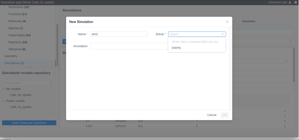
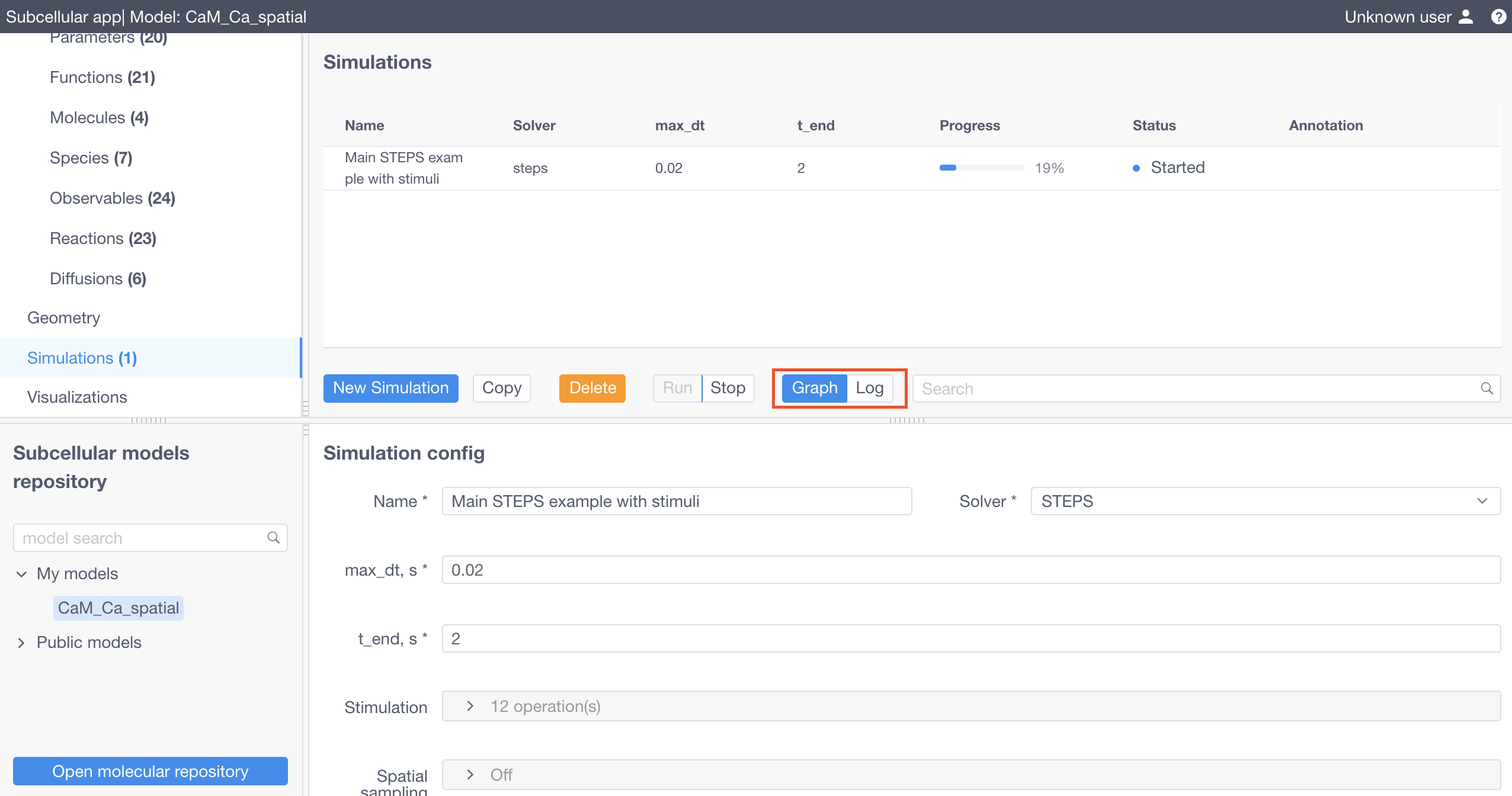
To simulate a model select Simulations on the Model panel, then create new simulation by clicking the corresponding button.
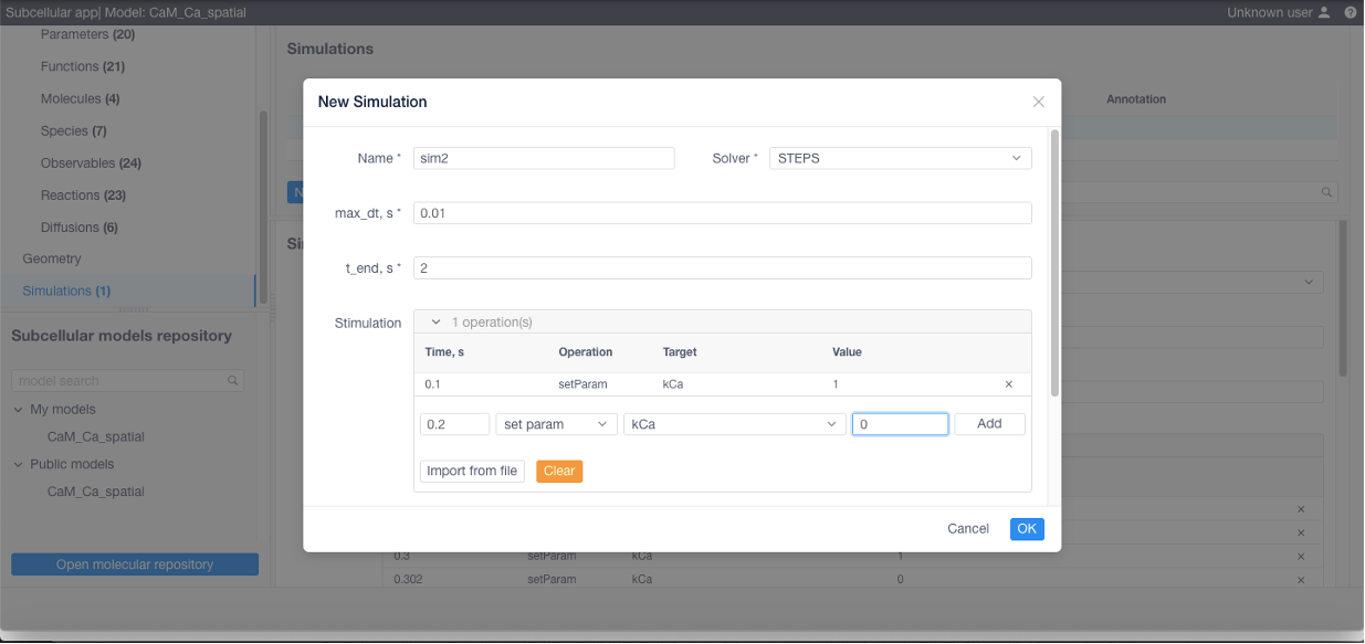
If desired add stimulations (this can be imported from a CSV or NFSim .rnf file) if needed:
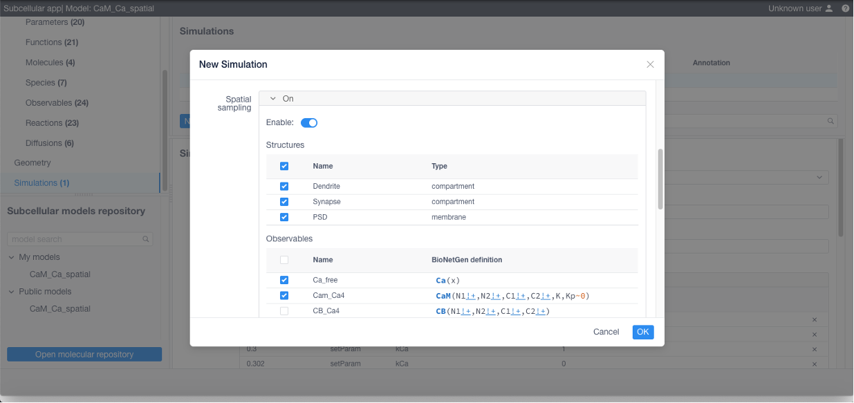
If 3D visualization is needed, Spatial sampling parameters (sampled compartments and observables) should be specified:
Click Apply in the bottom of the form and finally Run to start the simulation.

Simulation logs and charts are available for inspection once the simulation is started by clicking on Graph or Log buttons.
Example
Parameters
fac       1
kCa       0 * fac
Ca_in     0.08e-6 * 83.3 * fac
Ca_out    83.3 * fac
CBN1_on   75000000 * fac
CBN2_on   75000000 * fac
CBC1_on   75000000 * fac
CBC2_on   75000000 * fac
CBN1_off  29.5 * fac
CBN2_off  29.5 * fac
CBC1_off  29.5 * fac
CBC2_off  29.5 * fac
CaMN1_on  770000000 * fac
CaMN2_on  32000000000 * fac
CaMC1_on  84000000 * fac
CaMC2_on  25000000 * fac
CaMN1_off 160000 * fac
CaMN2_off 22000 * fac
CaMC1_off 2600 * fac
CaMC2_off 6.5 * fac
Functions
k__5()  = Ca_in
k__6()  = Ca_out
k_4()   = CBN1_on
k_5()   = CBN2_on
k_6()   = CBC1_on
k_7()   = CBC2_on
k_9()   = CBN1_off
k_10()  = CBN2_off
k_11()  = CBC1_off
k_12()  = CBC2_off
k_14()  = CaMN1_on
k_15()  = CaMN2_on
k_16()  = CaMC1_on
k_17()  = CaMC2_on
k_19()  = CaMN1_off
k_20()  = CaMN2_off
k_21()  = CaMC1_off
k_22()  = CaMC2_off
k__9()  = kCa * 1e3
k__10() = 1000 / 50
k__11() = 10 * 2 * 700 / 40 / 50 * 1000
Structures
Dendrite 3 1.1649e-18
Synapse  3 3.9820e-19
PSD      2 3.8885e-13
Molecule types
Ca(x)
CaM(N1,N2,C1,C2,K,Kp~0~1)
CB(N1,N2,C1,C2)
NMDA(pore~C~O,ank~0~1)
Species
@Dendrite:Ca(x)                   8e-08
@Dendrite:CaM(N1,N2,C1,C2,K,Kp~0) 8e-05
@Dendrite:CB(N1,N2,C1,C2)         3e-05
@Synapse:Ca(x)                    8e-08
@Synapse:CaM(N1,N2,C1,C2,K,Kp~0)  8e-05
@Synapse:CB(N1,N2,C1,C2)          3e-05
@PSD:NMDA(pore~C,ank~1)           40.0
Reaction Rules
NMDA_opening:  @PSD:NMDA(pore~C) -> @PSD:NMDA(pore~O)                       k__9()
NMDA_closing:  @PSD:NMDA(pore~O) -> @PSD:NMDA(pore~C)                       k__10()
NMDA_Ca_input: @PSD:NMDA(pore~O) -> @PSD:NMDA(pore~O) + @Synapse:Ca(x)      k__11()
Ca_input:      0 -> @Dendrite:Ca(x)                                         k__5()
Ca_extr:       @Dendrite:Ca(x) -> 0                                         k__6()
Ca_input1:     0 -> @Synapse:Ca(x)                                          k__5()
Ca_extr1:      @Synapse:Ca(x) -> 0                                          k__6()
N1_Ca_on:      CaM(N2,N1,K,Kp~0) + Ca(x) -> CaM(N2,N1!1,K,Kp~0).Ca(x!1)     k_14()
N2_Ca_on:      CaM(N1!+,N2,K,Kp~0) + Ca(x) -> CaM(N1!+,N2!1,K,Kp~0).Ca(x!1) k_15()
C1_Ca_on:      CaM(C2,C1,K,Kp~0) + Ca(x) -> CaM(C2,C1!1,K,Kp~0).Ca(x!1)     k_16()
C2_Ca_on:      CaM(C1!+,C2,K,Kp~0) + Ca(x) -> CaM(C1!+,C2!1,K,Kp~0).Ca(x!1) k_17()
N1_Ca_off:     CaM(N1!1,N2,K,Kp~0).Ca(x!1) -> CaM(N1,N2,K,Kp~0) + Ca(x)     k_19()
N2_Ca_off:     CaM(N1!+,N2!1,K,Kp~0).Ca(x!1) -> CaM(N1!+,N2,K,Kp~0) + Ca(x) k_20()
C1_Ca_off:     CaM(C1!1,C2,K,Kp~0).Ca(x!1) -> CaM(C1,C2,K,Kp~0) + Ca(x)     k_21()
C2_Ca_off:     CaM(C1!+,C2!1,K,Kp~0).Ca(x!1) -> CaM(C1!+,C2,K,Kp~0) + Ca(x) k_22()
CB_N1_Ca_on:   CB(N2,N1) + Ca(x) -> CB(N2,N1!1).Ca(x!1)                     k_4()
CB_N2_Ca_on:   CB(N1!+,N2) + Ca(x) -> CB(N2!1,N1!+).Ca(x!1)                 k_5()
CB_C1_Ca_on:   CB(C2,C1) + Ca(x) -> CB(C2,C1!1).Ca(x!1)                     k_6()
CB_C2_Ca_on:   CB(C1!+,C2) + Ca(x) -> CB(C1!+,C2!1).Ca(x!1)                 k_7()
CB_N1_Ca_off:  CB(N1!1,N2).Ca(x!1) -> CB(N1,N2) + Ca(x)                     k_9()
CB_N2_Ca_off:  CB(N1!+,N2!1).Ca(x!1) -> CB(N1!+,N2) + Ca(x)                 k_10()
CB_C1_Ca_off:  CB(C1!1,C2).Ca(x!1) -> CB(C1,C2) + Ca(x)                     k_11()
CB_C2_Ca_off:  CB(C1!+,C2!1).Ca(x!1) -> CB(C1!+,C2) + Ca(x)                 k_12()
Geometry specification (geometry.json)
{
  "meshNameRoot": "spine",
  "scale": 1e-06,
  "structures": [
    { "tetIdxs": [0, 1, 2, 3], "type": "compartment", "name": "Dendrite" },
    { "tetIdxs": [5, 15, 17, 18, 20, 25], "type": "compartment", "name": "Synapse"},
    { "triIdxs": [133, 141], "type": "membrane", "name": "PSD" }
  ],
  "freeDiffusionBoundaries": [{ "triIdxs": [203, 350], "name": "diffb_0" }]
}
Simulation config
max_dt: 0.02
t_end:  2
solver: STEPS
Stimulation
0.1   setParam kCa 1
0.105 setParam kCa 0
0.3   setParam kCa 1
0.302 setParam kCa 0
0.5   setParam kCa 1
0.502 setParam kCa 0
0.7   setParam kCa 1
0.702 setParam kCa 0
0.9   setParam kCa 1
0.902 setParam kCa 0
1.1   setParam kCa 1
1.102 setParam kCa 0
The above mentioned model with geometry and simulation configuration can be found in Public models as CaM_Ca_spatial model.
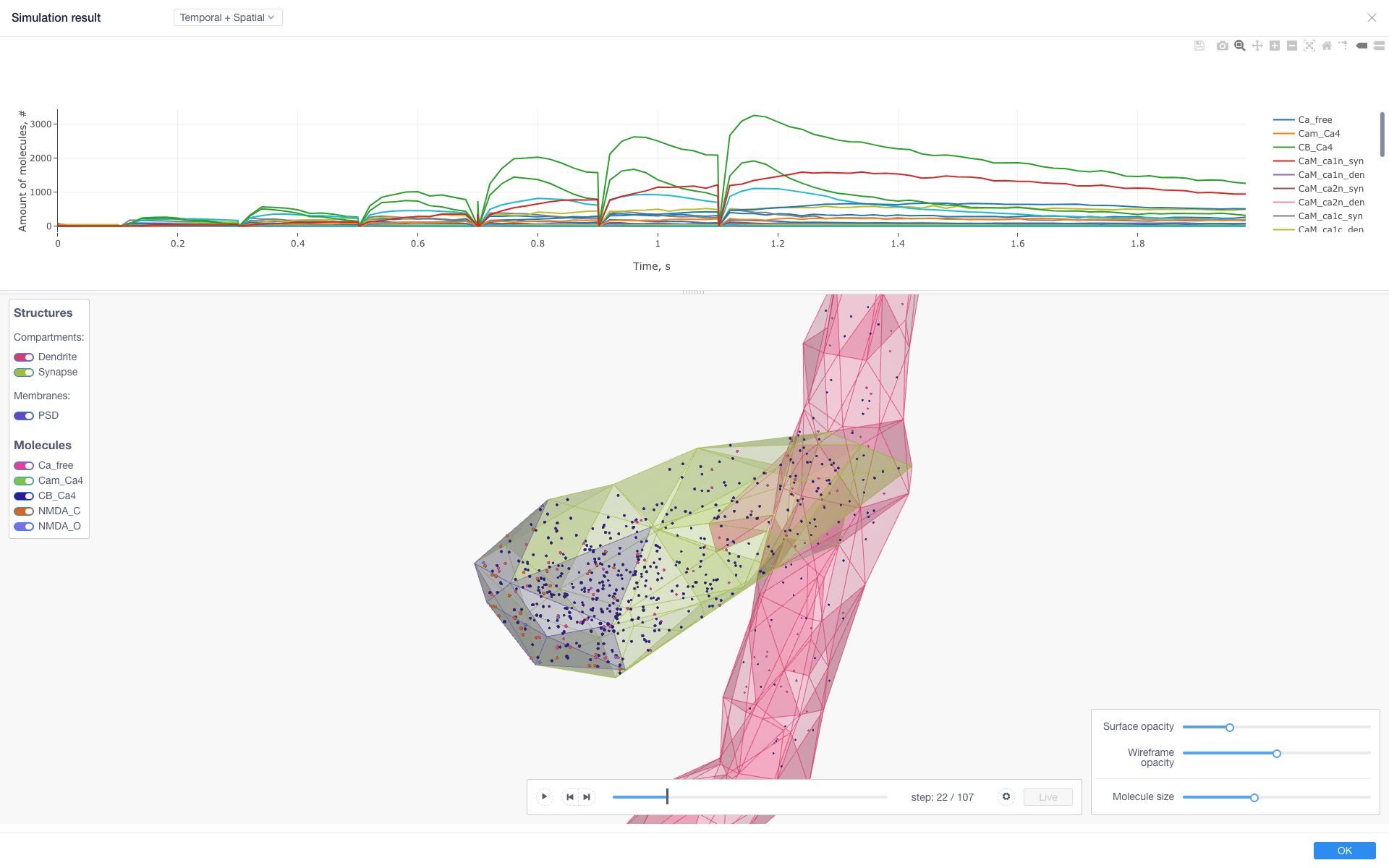
Results
Simulation results (available when sim has been started with live updates) can be downloaded as well as inspected with integrated:
cumulative per-observable concentration chart
spatial molecule distribution visualizer