Synaptic events fitting
This Use Case allows a user to fit synaptic events using data and models from the CSCS storage.
Selecting this Use Case, two Jupyter Notebooks are cloned in a private existing/new Collab. The cloned Notebooks are:
Synaptic events fitting - Config
It allows the user to:
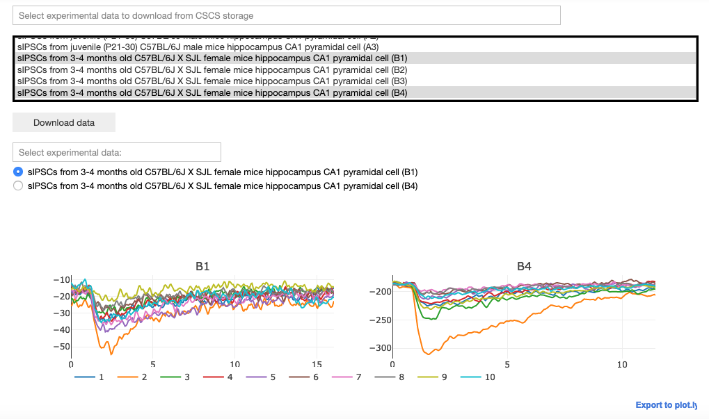
Select, download and visualize experimental data from the CSCS storage. The user may then select the data to be fitted.
A configuration file corresponding to the selected experimental file is downloaded from the Collab storage. This file includes: the number of traces in the experimental file, the protocol (voltage clamp amplitude and reversal potential of the synapse), the name of the parameters to be fitted, their initial values and the allowed variation range, exclusion rules, and an optional set of dependencies for other parameters
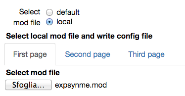
Select a default or a local mod file
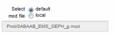
We assume that the user knows what we are talking about here, and that the uploaded mod file has been already tested by the user in preliminary simulations. The program does not check this. An invalid file will result in errors at NEURON compilation time
When a local mod file is chosen, a form with the values needed to write a corresponding configuration file is opened. The number of traces in the experimental file and the protocol (voltage clamp amplitude and reversal potential of the synapse) are by default filled with the values corresponding to the chosen experimental file. The name of the parameters to be fitted, their initial values and allowed variation range, exclusion rules, and an optional set of dependencies for other parameters must be filled in by the user. Typical values are shown in the figures below:
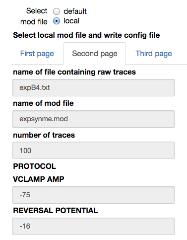
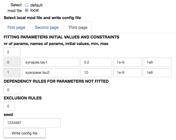
All other parameters that are not fitted have their default value as defined in the mod file.
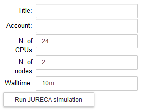
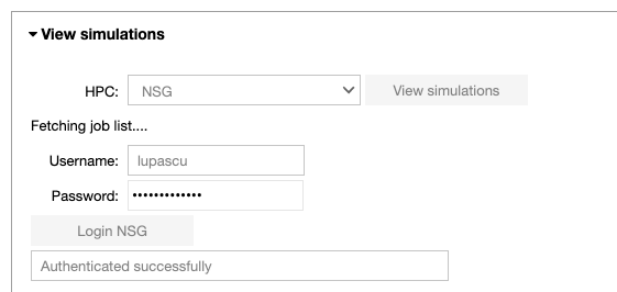
Configure the parameters of the optimization job: the title of the job, the number of nodes, the number of cores and the runtime. Run the fitting procedure using UNICORE authentication on JURECA (booster partition), GALILEO, or on NSG (using your account or the Service Account), and check the job status.
On JURECA, the node number, the number of CPUs per node and the runtime are set by default to 2, 24 and 10m respectively.
On GALILEO, the node number, the number of CPUs per node and the runtime are set by default to 2, 36 and 10m respectively.
The user needs to be aware of resource limitations imposed by each HPC system.
On NSG, the node number, the number of cores and the runtime are set by default to 2, 24 and 0.5 (hours) respectively. The maximum node number per job is 72. If you would require more than 72 nodes, please contact nsghelp@sdsc.edu. The maximum number of cores required per node is 24.
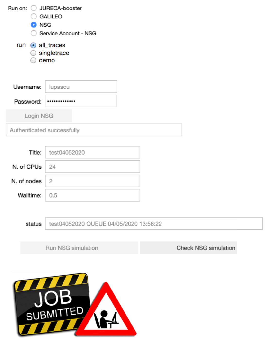
Note that when the job is submitted through UNICORE, the user can specify the project to use to submit the job on the HPC.
Note that when the job is submitted through NSG, next to the status of the job, the user may see the submission date converted to CET time. It will be useful in the analysis notebook in order to fetch the job.
The user can choose to fit all the experimental traces 100 times, a single trace 20 times or a demo version where a trace is fitted 5 times. For the single trace and the demo version the user can choose the number of the trace to be fitted.
Once the job is completed, the output files will be in the Collab storage under different directories, according to the system used.
JURECA: results are saved under the resultsJureca/jobtitle_fitting_submissionTime folder.
GALILEO: results are saved under the resultsGalileo/jobtitle_fitting_submissionTime folder.
NSG results are saved under the resultsNSG/jobtitle_fitting_submissionTime folder.
NSG (Service Account) results are saved under the resultsNSG-SA/jobtitle_fitting_submissionTime folder.
If you are interested in looking at the code, click on “Click here to toggle on/off the source code” button.

If you want to start a new fitting from the beginning, click on “Click here to start a new fit” button.

Synaptic events fitting - Analysis
This Jupyter Notebook allows the user to fetch the fitting results from the storage of the HPC system to the storage of the Collab or to analyze the optimized parameters. If the user wants to view an analysis of simulations that are already in the storage of the Collab, (s)he can skip the ‘View simulations’ tab and go directly to the ‘View analysis’ tab.
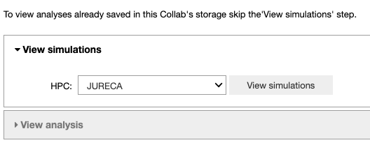
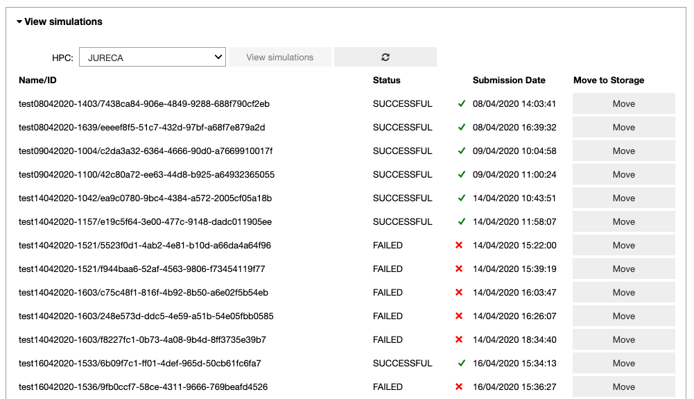
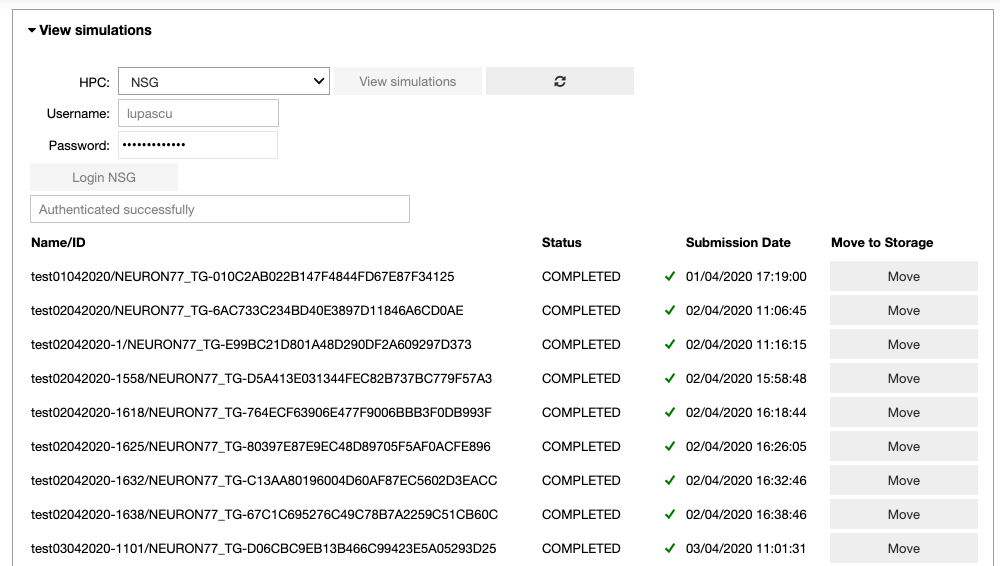
In the ‘View simulations’ tab, the user can visualize the Name/ID, status, the submission date of the simulations submitted on the HPC systems and (s)he can obtain an output of successfully completed jobs.
In the ‘View analysis’ tab, the user can analyze the optimized parameters for default data and a mod file combination or browse through the optimized parameters available in the Collab storage.
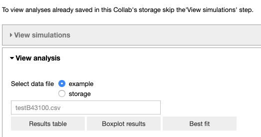
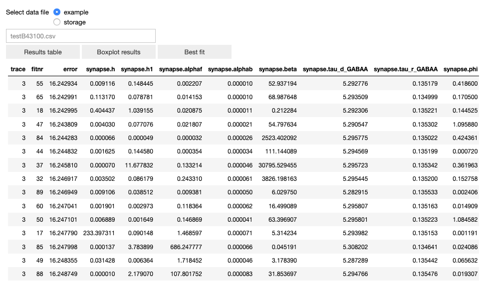
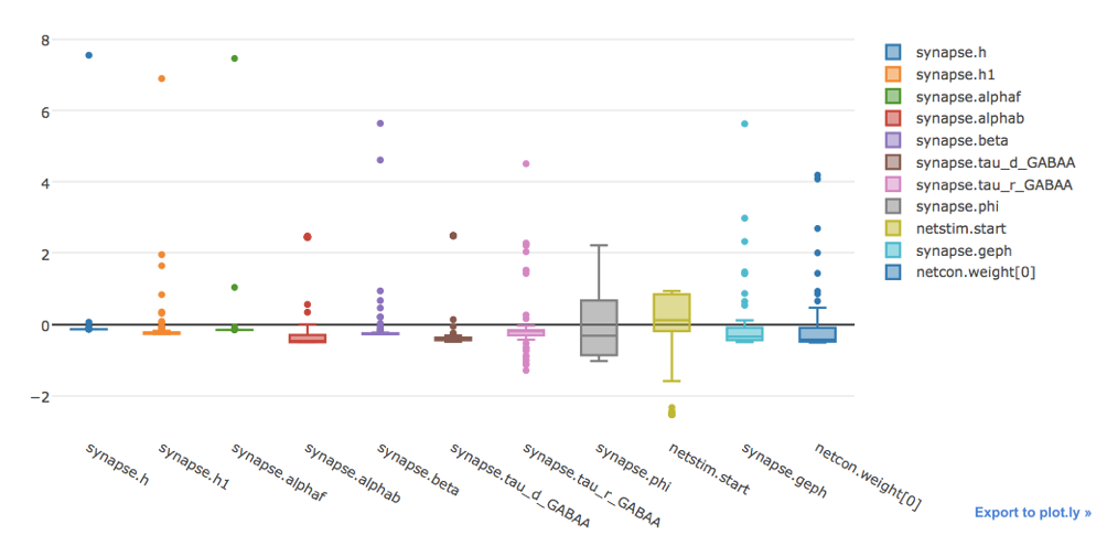
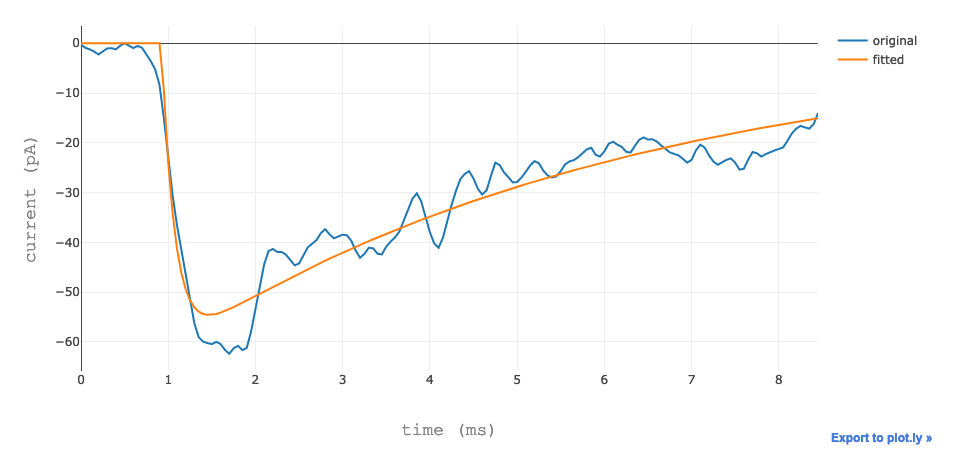
The user can visualize the data in table form, a box plot and the best fit.
The table of results (sorted in ascending order by the fitting error).
The boxplot of the normalized results.
The best fit.
If you are interested in the code, click on the “Click here to toggle on/off the source code” button.
